Are you enter the same section of data in different columns? Want to combine those columns in Microsoft 365 Excel and the older version MS Excel? You can easily combine columns in excel by merging cells. That means you can easily merge cells without losing data. When you use the “Merge&Center” option from the context menu, you will lose data. When you want to combine columns in excel without losing data you need to use a formula.
In this tutorial, I am going to show you two methods for combining columns in Excel. And I have provided a video tutorial for people who don’t want to spend much time and asking for reality.
- You May Like : How to split column in excel into multiple columns
- How to Insert Formula In Excel and Apply to Entire Column or Row
- 2 Simple Methods to Insert Excel into Word document
1. How to Combine columns in Microsoft 365 Excel?
Video Tutorial:
For our reader’s convenience, we have provided this article in video form. This video gives you more clarity in a realistic way. If you are willing to watch this video tutorial, click play. Otherwise, skip this video and continue reading.
Method 1:
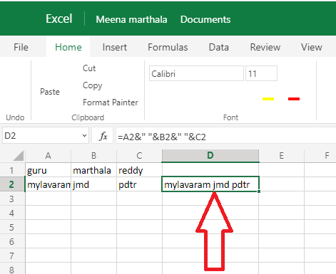
In this tutorial, we are going to see how to combine columns in an Excel sheet. We have mainly two types of excel sheets now-a-days. One is Microsoft 365 Excel and the other is an Older version MS Excel. In this section, first, we will see how to combine columns in Microsoft 365 Excel. Follow the below steps carefully.
Total Time: 4 minutes
Step 1: Open Excel sheet

Firstly, open the Excel sheet in Microsoft 365 in which you want to combine columns. Enter the data in different columns which you want to combine in another column.
Step 2: Enter Formula
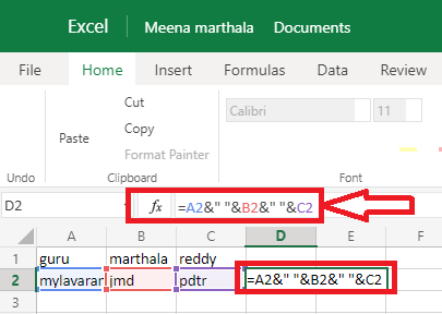
Now you will see the data in different columns in which you have entered previously. But we need all the data in different cells in a single cell. That means we need to combine the data. So we will search methods for combining those cells. Firstly we will use one formula for combining cells.
The formula that we use here is =A2&” “&B2&” “&C2. Place the cursor in the cell in which you want to get combined cell result. Now enter =A2&” “&B2&” “&C2 in the column where you want the combined result.
Step 3: Combined columns

Once you entered the formula in the specific cell and then click Enter. Then the data in cells will be combined. And that result will appear in the cell where you have placed the cursor.
If you want to combine columns in multiple rows, you don’t need to enter the formula again and again. just place the cursor at the first result, once you see the plus (+) symbol then drag the mouse. Then columns will combined in all rows. (This feature is shown in a realistic manner in the video tutorial)
* Type =A2&” “&B2&” “&C2 for separating words with a space.
* Type =A2&”,”&B2&”,”&C2 for separating words with a comma.
* Type =A2&”.”&B2&”.”&C2 for separating words with a dot symbol.
This is the one method procedure for combining cells in an Excel sheet.
Method 2:
In the previous section, we have seen one method for combining columns. In this section, we will see another method. In this method, we don’t use Ampersand (&) symbol in the formula. Follow the below steps.
- The first thing you need to is open Excel sheet in Microsoft 365. In that, you can see the data in different columns or cells. Now place the cursor in the column where you want to see the combined result.
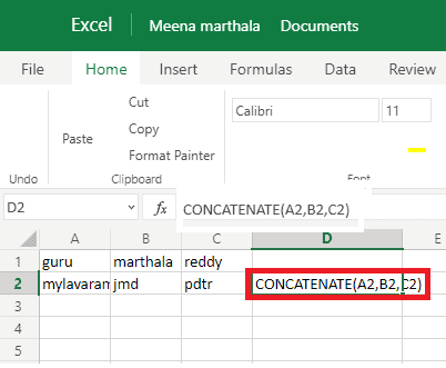
- Now enter =CONCATENATE(A2,B2,C2) and press Enter.
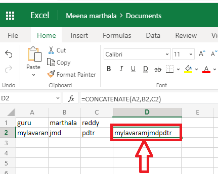
- Once you press enter then the data in different column cells will merge and the result will appear as shown in the above image.
- You can see some spaces and commas for separating those cell’s results.
- If you type =CONCATENATE(A2,B2,C2) then cell data will merge without any spaces.
- If you type =CONCATENATE(A2,”,”,B2,”,”,C2) then cell data will separated by commas.
- If you type =CONCATENATE(A2,”.”,B2,”.”,C2) then cell data will be separated by a dot symbol.
- This is the second method for combining columns in an Excel sheet.
2. How to combine columns in Older version MS Excel?
Note: It is not recommended to use the older version of word. We recommend buying Microsoft 365 for the best features.
Video Tutorial:
We are using the important formula to do this task. Make sure to watch a video, so that there would be no chance of mistake. However, we also have step-by-step instructions for you just after the video.
Here I am showing you two simple methods to Combine columns in excel by merging cells without losing data. You can use any one of the methods.
Method 1:
Combine columns in excel without space
Open your Excel sheet. Just see the below excel sheet. It has three columns (A, B, C). I am going to combine these three columns into one column (Column ‘E’).
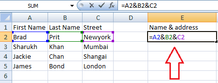
- In the above sheet real data starts from the 2nd row (A2, B2, C2). You need to merge A2, B2 & C2 cells.
- Click on the E2 cell. Type =A2&B2&C2 shows that in the above screenshot. (If your data starts from 1st row, you need to replace ‘2’ with ‘1’)
- Press “Enter”. You will see results in the E2 cell.
- Copy the E2 cell and paste it into the remaining cells. Or click at the right bottom of the E2 cell, hold the left click of a mouse, and drag to select the entire column. Immediately you will see the result in the entire column shows that in the below screenshot.

From the above picture, You can see that there is no space or any character between three words.
Combine columns in excel with space or special character
You can separate these three words with space or comma or dot or any other character.
- Use formula =A2&” “&B2&” “&C2 to separate words with space(there is a space between two colons and you can replace 2 with your corresponding row number).
- Use formula =A2&”,”&B2&”,”&C2 to separate words with comma.
- Use formula =A2&”.”&B2&”.”&C2 to separate words with a dot.
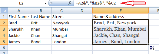
Likewise you can use any character between two colons to separate words.
Method 2:
You can use another formula to merge cells in excel.
Open excel sheet. Select E2 cell.
- Type =CONCATENATE(A2,B2,C2) to merge cells without space.
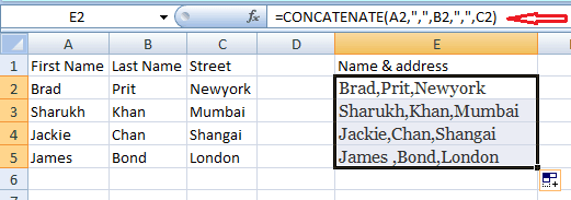
- Type =CONCATENATE(A2,”,”,B2,”,”,C2) to separate words with comma.
- Type =CONCATENATE(A2,”.”,B2,”.”,C2) to separate words with dot.
Press “Enter”. You will see result shows that in below screenshot. Copy same formula to entire column.
Conclusion:
We think now you might got complete details about How to combine columns in Microsoft 365 and older versions Excel. Once again we recommend to buy Microsoft 365. Because it gives you many features.
Thanks for reading my article about how to combine columns in excel. If you like it, do me favor by sharing it with your friends. You can also see the same procedure from Microsoft support topic. You can also follow whatvwant on Facebook and Twitter. Subscribe to whatVwant channel on YouTube for regular updates.
