
Want to split the columns in Excel? In this article, we are going to show you two methods one using Microsoft 365 Excel and the other method using the older version MS Office Excel.
While you are working with excel then there may be a need to split the columns. Then you must know how to do it. Do you know how to split columns in excel? If your answer is “No” then this article will help you a lot. Here I am giving the simple procedure to Split columns in excel into multiple columns. Suppose cells in a column of your excel sheet have a first name, last name, and date in a single cell separated with comma or tab or semicolon or etc, then you can easily convert them into multiple columns.
1. How to split columns into multiple columns in Microsoft 365 Excel?
Video Tutorial:
For our reader’s convenience, we have provided this article in the form of video tutorial. If you are willing to watch video tutorial, then click play. Otherwise skip this video, continue reading.
In this section, we will see how to split column into multiple columns.
Total Time: 4 minutes
Step 1: Open Excel
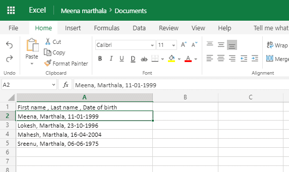
Firstly, open the Excel sheet in Microsoft 365. In that you can see number of cells with A, B, C, ……. which represent columns and 1, 2, 3, …… which represent rows.
Step 2: Click on Data
As a part of the Excel sheet editing, viewing you can see a list of options in the menu bar to make your excel sheet more stylish and easy to understand.
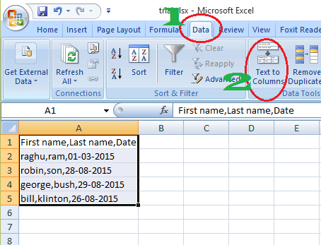
Here, I have data of four persons which contains first name, last name and date of birth in single column separated by commas. Now I need to split that column data into multiple columns that mean I want to see First name, last name and date of birth in different columns. So select the particular row of a column or you can select multiple rows at a time which you want to split
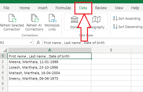
In the menu bar, you can see Data option in the fifth position from the left side of the screen. Click on that Data option.
Step 3: Click on Text to Columns
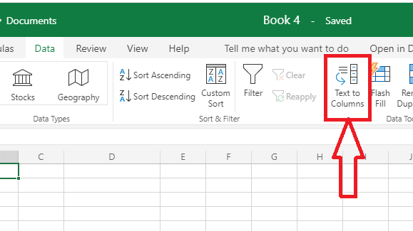
In the Data menu, you can see different options like Sort Ascending, Sort Descending, Custom sort, Filter, Flash fill, etc. On that screen, you can also see Text to Columns. Click on that Text to Columns.
Step 4: Select Delimiters
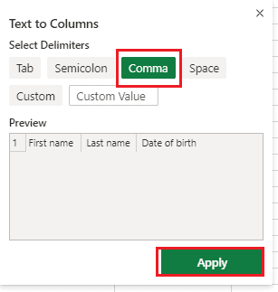
When you click on the Text to Columns, you can see the above screen. You need to select a Delimeter from the available options like Tab, Semicolon, Common and space. Here I have entered Comma so I selected the comma. You can see the preview also. And then click on Apply as shown in the above image.
Step 5: Result in different columns

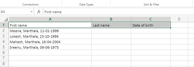
Once you click on Apply option, then you can see the data of same column split into different columns as shown in the image.
This is the procedure for splitting the same column data into different columns.
2. How to Split columns into multiple columns in Older version MS Office Excel?
Video Tutorial:
We provided this article in the form of a video tutorial for our reader’s convenience. If you are interested in reading, you can skip the video and start reading.
- Open your excel sheet.
- Select the entire column which you want to split. You can use a mouse or shift + down arrow to select the entire row.
- Click on “Data” in the top menu.
- Click “Text to Columns” shows that in the above screenshot. You will see another window shows that in the below screenshot.
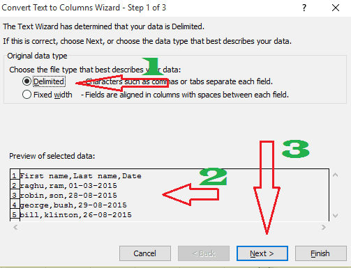
- Make sure you have selected “Delimited”.
- Check the preview of your selected date in the rectangular box. If anything goes wrong, you can reselect again.
- Click “Next”. You will see another window shows that in the below screenshot.
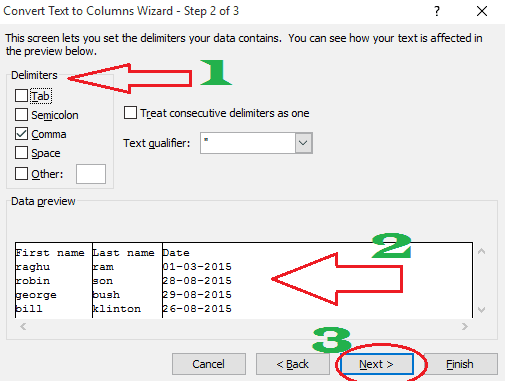
- Check any one of the options available under “Delimiters“. Here, I have selected “comma” because my data was separated with “comma”. If your data is separated with semicolon or tab or space you need to select options according to your data.
- Check your preview in the “Data preview” box.
- Click “Next” if you like the preview. You will see another window shows that in the below screenshot.

Check “Data Preview”, you will see your output columns. Click on the first column. Check the corresponding format under “Column Data Format”. In this example, the first column contains the first name which is a text. So I have selected “Text” under “Column Data Format”. The second column is also text. The third column is the date, so I have selected “Date”. Likewise, you can select a data format for all columns.
Now you need to select destination fields for your output. Click on the symbol right to the “Destination” field shows that in the above screenshot. You will see a small rectangular window shows that in the below screenshot.
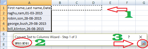
- Click on any cell and use the shift + right arrow mark to select cells where you want to place output data.
- You can check the selected columns in the wizard. Here I have selected cells B1, C1, and D1. Because my output has three columns. You can see the selection in the wizard B1 to D1.
- Click on the same symbol in the right bottom corner to close this wizard. You will go back to the main wizard.
Click “Finish” on the main wizard. You will see the output shows that in the below screenshot.

Here I have selected cells from B1 to D1. So my original data stays in A cell. If you had selected cells from A1 to C1 you will not see the original data. That will be overwritten by the output result.
Conclusion:
I think now you might know complete details about How to split column into multiple columns in Microsoft 365 and older versions. Once again we recommend to buy Microsoft 365. Because it gives you many features.
Thanks for reading my article about Split columns in excel into multiple columns. If you like it, do me favor by sharing it with your friends and follow WhatVwant on Facebook and Twitter for more tips. Subscribe to whatVwant channel on YouTube for regular updates.